---
title: "AERIS: Argonne's Earth Systems Model"
description: "Presentation at the 2025 ALCF Hands On HPC Workshop"
location: "[2025 ALCF Hands-on HPC Workshop](https://www.alcf.anl.gov/events/2025-alcf-hands-hpc-workshop)"
location-url: "https://www.alcf.anl.gov/events/2025-alcf-hands-hpc-workshop"
date: 2025-10-08
date-modified: last-modified
number-sections: false
image: ./assets/thumbnail.png
lightbox: auto
editor:
render-on-save: true
twitter-card:
image: ./assets/thumbnail.png
site: "saforem2"
creator: "saforem2"
title: "AERIS: Argonne Earth Systems Model for Reliable and Skillful Predictions"
description: "Presented at the 2025 ALCF Hands-on HPC Workshop."
open-graph:
title: "AERIS: Argonne Earth Systems Model for Reliable and Skillful Predictions"
description: "Presented at the 2025 ALCF Hands-on HPC Workshop."
image: "./assets/thumbnail.png"
citation:
author: Sam Foreman
type: speech
url: https://samforeman.me/talks/2025/10/08/slides.html
# toc-expand: true
aliases:
- /talks/2025/aeris/index.html
format:
html:
reader-mode: true
# toc-depth: 1
# grid:
# page-layout: full
# body-width: 1000px
# # margin-width: 250px
# # sidebar-width: 250px
# # gutter-width: 1.5rem
# shift-heading-level-by: 1
image: "./assets/thumbnail.png"
mermaid:
# theme: neutral
look: neo
layout: dagre
useMaxWidth: true
revealjs:
shift-heading-level-by: -1
image: "./assets/thumbnail.png"
footer: "[samforeman.me/talks/2025/10/08/slides](https://samforeman.me/talks/2025/10/08/slides.html)"
slide-url: https://samforeman.me/talks/2025/10/08/slides.html
mermaid:
layout: dagre
useMaxWidth: true
# title-slide-attributes:
title-slide-attributes:
data-background-image: ./assets/cover0.svg
data-background-size: contain
data-background-opacity: "0.5"
# data-background-color: "oklch(from #E599F7 l c * 1.15 h / 0.1)"
# aliases:
# - /talks/alcf-hands-on-hpc-2025/slides.html
gfm: default
---
## 🌎 AERIS {background-color="white"}
::: {.content-visible unless-format="revealjs"}
::: {.flex-container background-color="white"}
::: {.flex-child style="width:50%;"}
](./assets/team.png){#fig-arxiv}
:::
::: {.flex-child style="width:43.6%;"}

:::
:::
:::
::: {.content-visible when-format="revealjs"}
::: {.flex-container}
::: {.flex-child style="width:50%;"}
](./assets/team.png){#fig-arxiv}
:::
::: {.flex-child style="width:43.6%;"}
![Pixel-level Swin diffusion transformer in sizes from \[1--80\]B](./assets/cover2.svg)
:::
:::
:::
::: notes
> We demonstrate a significant advancement in AI weather
> and climate modeling with AERIS by efficient scaling of
> window-based transformer models. We have performed global
> medium-range forecasts with performance competitive with
> GenCast and surpassing the IFS ENS model, with longer, 90-
> day rollouts showing our ability to learn atmospheric dynamics
> on seasonal scales without collapsing, becoming the first
> diffusion-based model that can work across forecast scales
> from 6 hours all the way to 3 months with remarkably accurate
> out of distribution predictions of extreme events.
:::
## High-Level Overview of AERIS {.smaller background-color="white"}
::: {.flex-container}
::: {#fig-rollout}
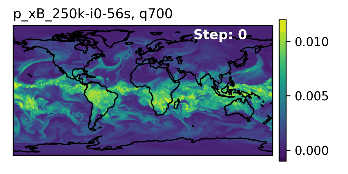
Rollout of AERIS model, specific humidity at 700m.
:::
::: {#tbl-aeris}
| Property | Description |
| -----------------: | :---------------- |
| Domain | Global |
| Resolution | 0.25° \& 1.4° |
| Training Data | ERA5 (1979--2018) |
| Model Architecture | Swin Transformer |
| Speedup[^pde] | O(10k--100k) |
: Overview of AERIS model and training setup {.responsive .striped .hover}
:::
:::
[^pde]: Relative to PDE-based models, e.g.: [GFS](https://www.ncdc.noaa.gov/data-access/model-data/model-datasets/global-forcast-system-gfs)
## Contributions {background-color="white"}
::: {.flex-container}
::: {.callout-caution icon=false title="☔ AERIS"}
_First billion-parameter diffusion model for weather \+ climate_
- Operates at the pixel level (1 × 1 patch size)
- Guided by physical priors
- Medium-range forecast skill
- Surpasses IFS ENS, competitive with GenCast (@price2024gencast)
- Uniquely stable on seasonal scales to 90 days
:::
::: {.callout-note icon=false title="🌀 SWiPe"}
- SWiPe, _novel_ 3D (sequence-window-pipeline) parallelism strategy for training
transformers across high-resolution inputs
- Enables scalable small-batch training on large supercomputers[^aurora-scale]
- **10.21 ExaFLOPS** @ 121,000 Intel XPUs (Aurora)
:::
:::
[^aurora-scale]: Demonstrated on up to 120,960 GPUs on Aurora and 8,064 GPUs on LUMI.
## Model Overview {background-color="white"}
::: {.flex-container style="align-items: flex-start;"}
::: {#tbl-data-vars}
| Variable | Description |
| :-----------:| :---------------------------- |
| `t2m` | 2m Temperature |
| `X` `u`(`v`) | $u$ ($v$) wind component @ Xm |
| `q` | Specific Humidity |
| `z` | Geopotential |
| `msl` | Mean Sea Level Pressure |
| `sst` | Sea Surface Temperature |
| `lsm` | Land-sea mask |
: Variables used in AERIS training and prediction {.responsive .striped .hover}
:::
::: {.flex-child}
- **Dataset**: ECMWF Reanalysis v5 (ERA5)
- **Variables**: Surface and pressure levels
- **Usage**: Medium-range weather forecasting
- **Partition**:
- Train: 1979--2018[^days]
- Val: 2019
- Test: 2020
- **Data Size**: 100GB at 5.6° to 31TB at 0.25°
:::
[^days]: ~ 14,000 days of data
:::
## Windowed Self-Attention {.smaller background-color="white"}
::: {.flex-container}
::: {.flex-child style="width:33%;"}
- **Benefits for weather modeling**:
- Shifted windows capture both local patterns and long-range context
- Constant scale, windowed self-attention provides high-resolution forecasts
- Designed (currently) for fixed, 2D grids
- **Inspiration from SOTA LLMs**:
- `RMSNorm`, `SwiGLU`, 2D `RoPE`
:::
::: {#fig-windowed-self-attention style="width:66%;"}
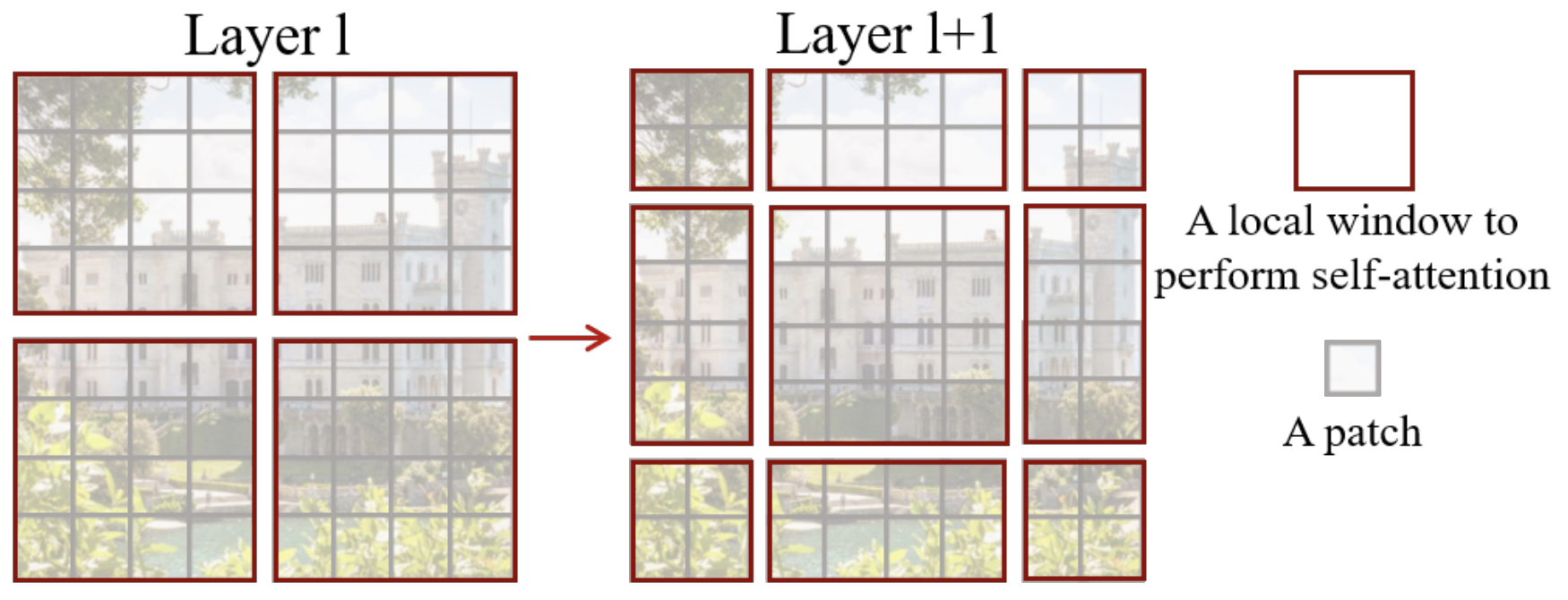
Windowed Self-Attention
:::
:::
## Model Architecture: Details {background-color="white"}
::: {.content-visible unless-format="revealjs"}
::: {#fig-model-arch-details style="width:80%; text-align: center; margin-left: auto; margin-right: auto;"}

Model Architecture
:::
:::
::: {.content-visible when-format="revealjs"}
::: {#fig-swipe-layer style="width:90%; text-align: center; margin-left: auto; margin-right: auto;"}

Model Architecture
:::
:::
## Issues with the Deterministic Approach {background-color="white"}
::: {.flex-container}
::: {.flex-child}
- [{{< iconify material-symbols close>}}]{.red-text} [**Transformers**]{.highlight-red}:
- *Deterministic*
- Single input → single forecast
:::
::: {.flex-child}
<!-- {{< iconify ph github-logo-duotone >}} -->
- [{{<iconify material-symbols check>}}]{.green-text} [**Diffusion**]{.highlight-green}:
- *Probabilistic*
- Single input → _**ensemble of forecasts**_
- Captures uncertainty and variability in weather predictions
- Enables ensemble forecasting for better risk assessment
:::
:::
## Transitioning to a Probabilistic Model {background-color="white"}
::: {#fig-forward-pass}

Reverse diffusion with the [input]{style="color:#228be6"} condition, individual
sampling steps $t_{0} \rightarrow t_{64}$, the next time step
[estimate]{style="color:#40c057"} and the [target]{style="color:#fa5252"}
output.
:::
::: {.flex-container}
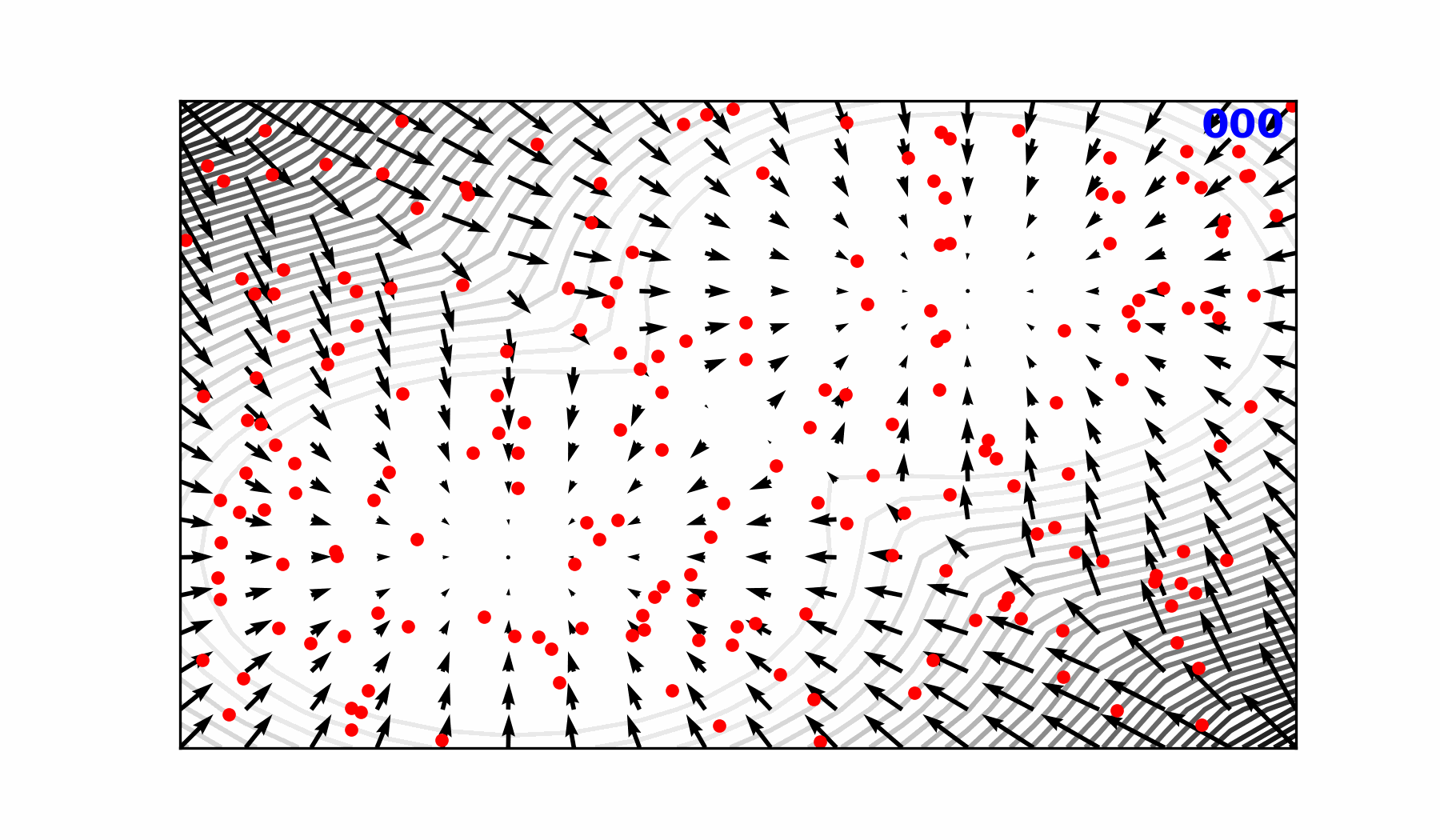
{width="89.6%"}
:::
## Sequence-Window-Pipeline Parallelism `SWiPe` {.smaller background-color="white"}
::: {.content-visible unless-format="revealjs"}
::: {.flex-container}
::: {.flex-child style="width:33%;"}
- `SWiPe` is a **novel parallelism strategy** for Swin-based Transformers
- Hybrid 3D Parallelism strategy, combining:
- Sequence parallelism (`SP`)
- Window parallelism (`WP`)
- Pipeline parallelism (`PP`)
:::
::: {#fig-swipe-layer style="width:66%;"}

:::
:::
::: {#fig-comms style="width:80%; text-align: center; margin-left: auto; margin-right: auto; "}

`SWiPe` Communication Patterns
:::
:::
::: {.content-visible when-format="revealjs"}
::: {.flex-container}
::: {.flex-child style="width:33%;"}
- `SWiPe` is a **novel parallelism strategy** for Swin-based Transformers
- Hybrid 3D Parallelism strategy, combining:
- Sequence parallelism (`SP`)
- Window parallelism (`WP`)
- Pipeline parallelism (`PP`)
:::
::: {#fig-swipe-layer style="width:66%;"}

:::
:::
::: {#fig-comms style="width:60%; text-align: center; margin-left: auto; margin-right: auto;"}

`SWiPe` Communication Patterns
:::
:::
## Aurora {background-color="white" style="width:100%"}
::: {.flex-container style="align-items: center; gap:10pt;"}
::: {.column #tbl-aurora}
| Property | Value |
| -----------: | :------ |
| Racks | 166 |
| Nodes | 10,624 |
| XPUs[^tiles] | 127,488 |
| CPUs | 21,248 |
| NICs | 84,992 |
| HBM | 8 PB |
| DDR5c | 10 PB |
: Aurora[^aurora-ai] Specs {.responsive .striped .hover}
:::
::: {#fig-aurora .r-stretch}

Aurora: [Fact Sheet](https://www.alcf.anl.gov/sites/default/files/2024-07/Aurora_FactSheet_2024.pdf).
:::
:::
[^tiles]: Each node has 6 Intel Data Center GPU Max 1550
(code-named "Ponte Vecchio") tiles, with 2 XPUs per tile.
[^aurora-ai]: 🏆 [Aurora Supercomputer Ranks Fastest for AI](https://www.intel.com/content/www/us/en/newsroom/news/intel-powered-aurora-supercomputer-breaks-exascale-barrier.html)
## AERIS: Scaling Results {background-color="white"}
::: {.flex-container}
::: {.column #fig-aeris-scaling style="width:70%;"}

AERIS: Scaling Results
:::
::: {.column style="width:30%;"}
- [**10 EFLOPs**]{.highlight-blue} (sustained) @ **120,960 GPUs**
- See (@stock2025aeris) for additional details
- [arXiv:2509.13523](https://arxiv.org/abs/2509.13523)
:::
:::
## Hurricane Laura {background-color="white"}
::: {#fig-hurricane-laura}
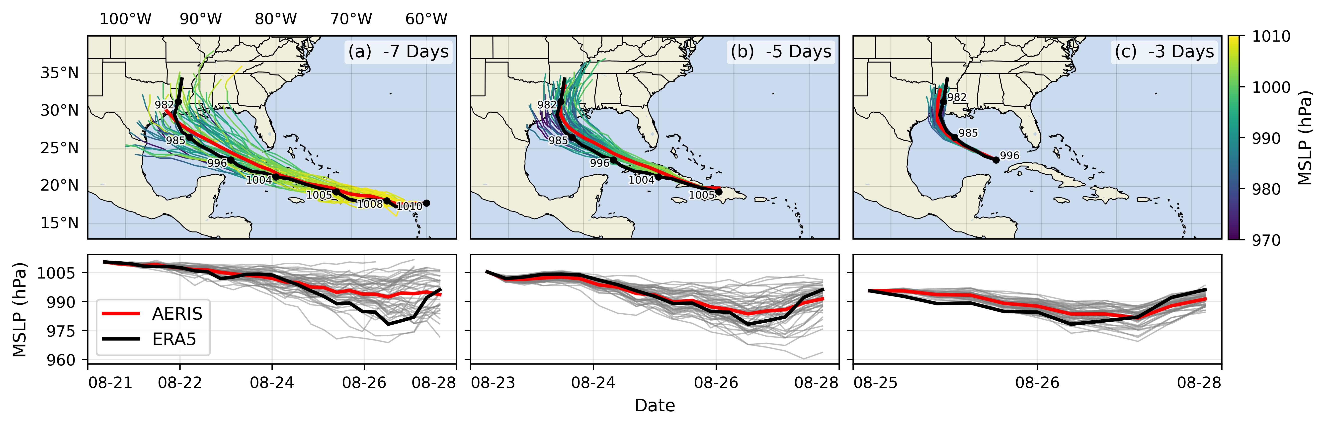
Hurricane Laura tracks (top) and intensity (bottom). Initialized 7(a), 5(b) and
3(c) days prior to 2020-08-28T00z.
:::
## S2S: Subsseasonal-to-Seasonal Forecasts {.smaller background-color="white"}
::: {.flex-container}
::: {.callout-important icon=false title="🌡️ S2S Forecasts"}
We demonstrate for the first time, the ability of a generative, high
resolution (native ERA5) diffusion model to produce skillful forecasts on the
S2S timescales with realistic evolutions of the Earth system
(atmosphere + ocean).
:::
::: {.flex-child}
- To assess trends that extend beyond that of our medium-range weather forecasts
(beyond 14-days) and evaluate the stability of our model, we made 3,000
forecasts (60 initial conditions each with 50 ensembles) out to 90 days.
- AERIS was found to be stable during these 90-day forecasts
- Realistic atmospheric states
- Correct power spectra even at the smallest scales
:::
:::
## Seasonal Forecast Stability {.smaller background-color="white"}
::: {#fig-seasonal-forecast-stability style="text-align: center; margin-left: auto; margin-right: auto;"}
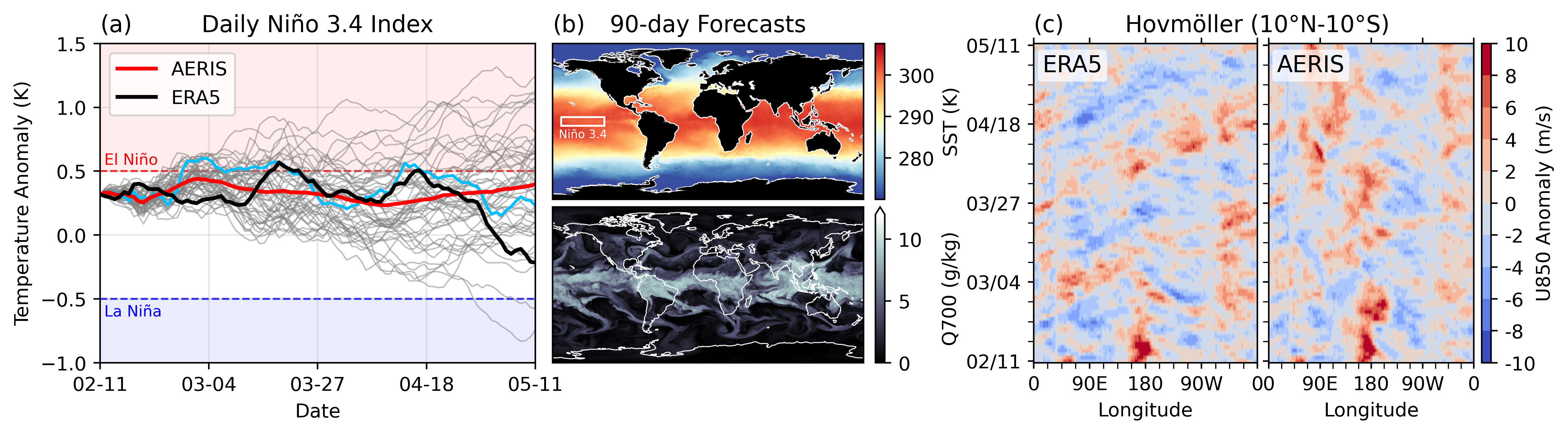
S2S Stability: (a) Spring barrier El Niño with realistic ensemble spread in the
ocean; (b) qualitatively sharp fields of SST and Q700 predicted 90 days in the
future from the [closest]{style="color:#65B8EE;"} ensemble member to the ERA5
in (a); and (c) stable Hovmöller diagrams of U850 anomalies (climatology
removed; m/s), averaged between 10°S and 10°N, for a 90-day rollout.
:::
## Next Steps {background-color="white"}
- [Swift](https://github.com/stockeh/swift): Swift, a single-step consistency
model that, for the first time, enables autoregressive finetuning of a
probability flow model with a continuous ranked probability score (CRPS)
objective
## References {background-color="white"}
1. [What are Diffusion Models? | Lil'Log](https://lilianweng.github.io/posts/2021-07-11-diffusion-models/)
1. [Step by Step visual introduction to Diffusion Models. - Blog by Kemal Erdem](https://erdem.pl/2023/11/step-by-step-visual-introduction-to-diffusion-models)
1. [Understanding Diffusion Models: A Unified Perspective](https://calvinyluo.com/2022/08/26/diffusion-tutorial.html)
::: {#refs}
:::
## Extras
### Overview of Diffusion Models
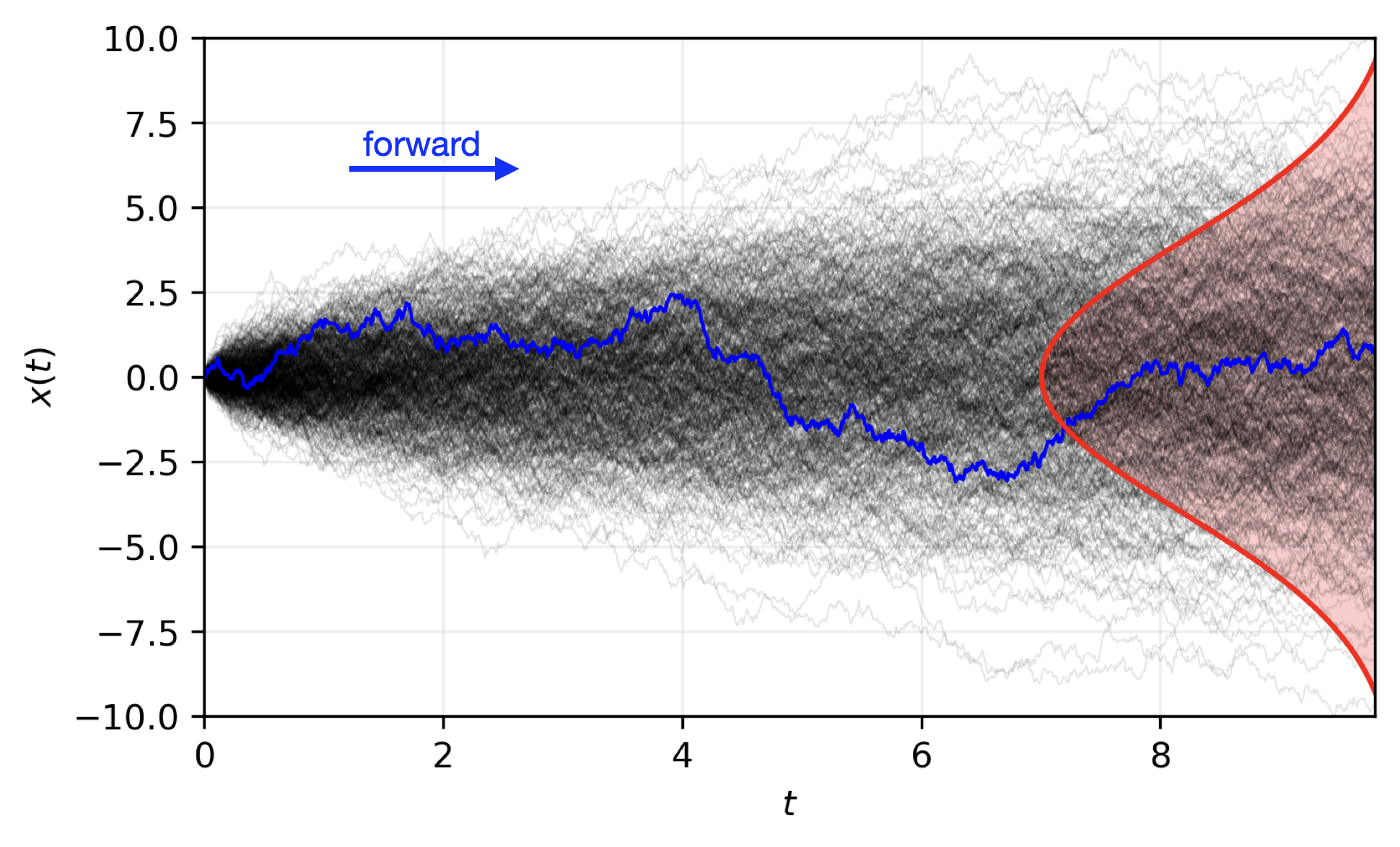
**Goal**: We would like to (efficiently) draw samples $x_{i}$ from a
(potentially unknown) _target_ distribution $q(\cdot)$.
- Given $x_{0} \sim q(x)$, we can construct a _forward diffusion process_ by
gradually adding noise to $x_{0}$ over $T$ steps:
$x_{0} \rightarrow \left\{x_{1}, \ldots, x_{T}\right\}$.
- Step sizes $\beta_{t} \in (0, 1)$ controlled by a _variance schedule_
$\{\beta\}_{t=1}^{T}$, with:
$$\begin{aligned}
q(x_{t}|x_{t-1}) = \mathcal{N}(x_{t}; \sqrt{1-\beta_{t}} x_{t-1}, \beta_{t} I) \\
q(x_{1:T}|x_{0}) = \prod_{t=1}^{T} q(x_{t}|x_{t-1})
\end{aligned}$$
### Diffusion Model: Forward Process
- Introduce:
- $\alpha_{t} \equiv 1 - \beta_{t}$
- $\bar{\alpha}_{t} \equiv \prod_{s=1}^{T} \alpha_{s}$
We can write the forward process as:
$$ q(x_{1}|x_{0}) = \mathcal{N}(x_{1}; \sqrt{\bar{\alpha}_{1}} x_{0}, (1-\bar{\alpha}_{1}) I)$$
- We see that the _mean_ $\mu_{t} = \sqrt{\alpha_{t}} x_{t-1} = \sqrt{\bar{\alpha}_{t}} x_{0}$
## Acknowledgements {background-color="white"}
> This research used resources of the Argonne Leadership Computing
> Facility, which is a DOE Office of Science User Facility supported
> under Contract DE-AC02-06CH11357.