AERIS: Argonne’s Earth Systems Model

Sam Foreman

[email protected]

ALCF

2025-10-08

🌎 AERIS

Figure 1: arXiv:2509.13523

Pixel-level Swin diffusion transformer in sizes from [1–80]B

We demonstrate a significant advancement in AI weather and climate modeling with AERIS by efficient scaling of window-based transformer models. We have performed global medium-range forecasts with performance competitive with GenCast and surpassing the IFS ENS model, with longer, 90- day rollouts showing our ability to learn atmospheric dynamics on seasonal scales without collapsing, becoming the first diffusion-based model that can work across forecast scales from 6 hours all the way to 3 months with remarkably accurate out of distribution predictions of extreme events.

High-Level Overview of AERIS

Figure 2: Rollout of AERIS model, specific humidity at 700m.

Table 1: Overview of AERIS model and training setup

Property	Description
Domain	Global
Resolution	0.25° & 1.4°
Training Data	ERA5 (1979–2018)
Model Architecture	Swin Transformer
Speedup1	O(10k–100k)

1. Relative to PDE-based models, e.g.: GFS

Contributions

☔ AERIS

First billion-parameter diffusion model for weather + climate

• Operates at the pixel level (1 × 1 patch size)
• Guided by physical priors
• Medium-range forecast skill
  • Surpasses IFS ENS, competitive with GenCast (Price et al. (2024))
  • Uniquely stable on seasonal scales to 90 days

🌀 SWiPe

• SWiPe, novel 3D (sequence-window-pipeline) parallelism strategy for training transformers across high-resolution inputs
  • Enables scalable small-batch training on large supercomputers¹
    • 10.21 ExaFLOPS @ 121,000 Intel XPUs (Aurora)

1. Demonstrated on up to 120,960 GPUs on Aurora and 8,064 GPUs on LUMI.

Model Overview

Table 2: Variables used in AERIS training and prediction

Variable	Description
t2m	2m Temperature
X u(v)	u (v) wind component @ Xm
q	Specific Humidity
z	Geopotential
msl	Mean Sea Level Pressure
sst	Sea Surface Temperature
lsm	Land-sea mask

• Dataset: ECMWF Reanalysis v5 (ERA5)
• Variables: Surface and pressure levels
• Usage: Medium-range weather forecasting
• Partition:
  • Train: 1979–2018¹
  • Val: 2019
  • Test: 2020
• Data Size: 100GB at 5.6° to 31TB at 0.25°

1. ~ 14,000 days of data

Windowed Self-Attention

• Benefits for weather modeling:
  • Shifted windows capture both local patterns and long-range context
  • Constant scale, windowed self-attention provides high-resolution forecasts
  • Designed (currently) for fixed, 2D grids
• Inspiration from SOTA LLMs:
  • RMSNorm, SwiGLU, 2D RoPE

Figure 3: Windowed Self-Attention

Model Architecture: Details

Figure 4: Model Architecture

Issues with the Deterministic Approach

• Transformers:
  • Deterministic
  • Single input → single forecast

• Diffusion:
  • Probabilistic
  • Single input → ensemble of forecasts
  • Captures uncertainty and variability in weather predictions
  • Enables ensemble forecasting for better risk assessment

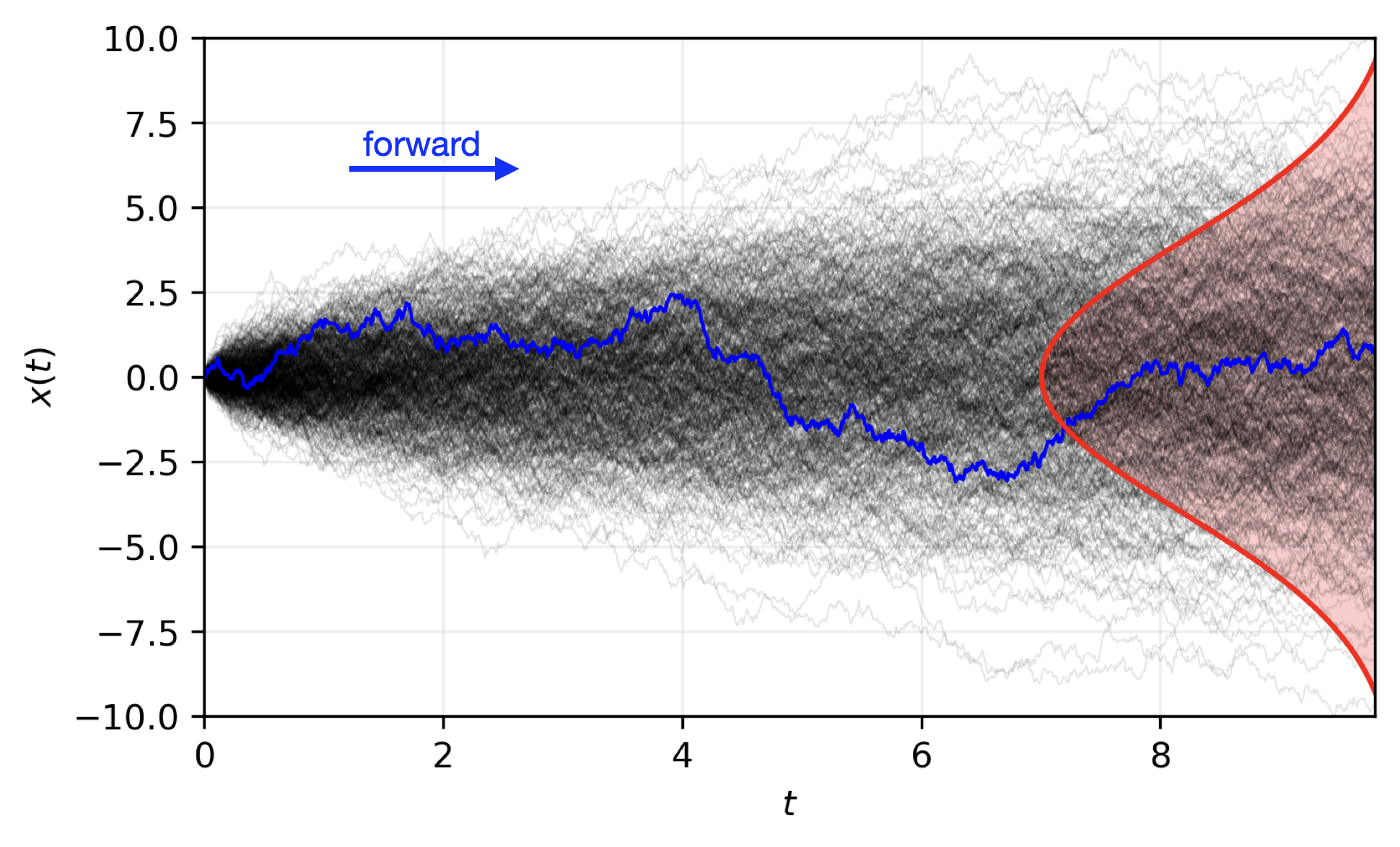
Transitioning to a Probabilistic Model

Figure 5: Reverse diffusion with the input condition, individual sampling steps t_{0} \rightarrow t_{64}, the next time step estimate and the target output.

Reverse Diffusion Process (\mathcal{N}\rightarrow \pi)

Forward Diffusion Process (\pi\rightarrow \mathcal{N})

Sequence-Window-Pipeline Parallelism SWiPe

• SWiPe is a novel parallelism strategy for Swin-based Transformers
• Hybrid 3D Parallelism strategy, combining:
  • Sequence parallelism (SP)
  • Window parallelism (WP)
  • Pipeline parallelism (PP)

Figure 6

Figure 7: SWiPe Communication Patterns

Aurora

Table 3: Aurora¹ Specs

Property	Value
Racks	166
Nodes	10,624
XPUs2	127,488
CPUs	21,248
NICs	84,992
HBM	8 PB
DDR5c	10 PB

Figure 8: Aurora: Fact Sheet.

1. 🏆 Aurora Supercomputer Ranks Fastest for AI

2. Each node has 6 Intel Data Center GPU Max 1550 (code-named “Ponte Vecchio”) tiles, with 2 XPUs per tile.

AERIS: Scaling Results

Figure 9: AERIS: Scaling Results

• 10 EFLOPs (sustained) @ 120,960 GPUs
• See (Hatanpää et al. (2025)) for additional details
• arXiv:2509.13523

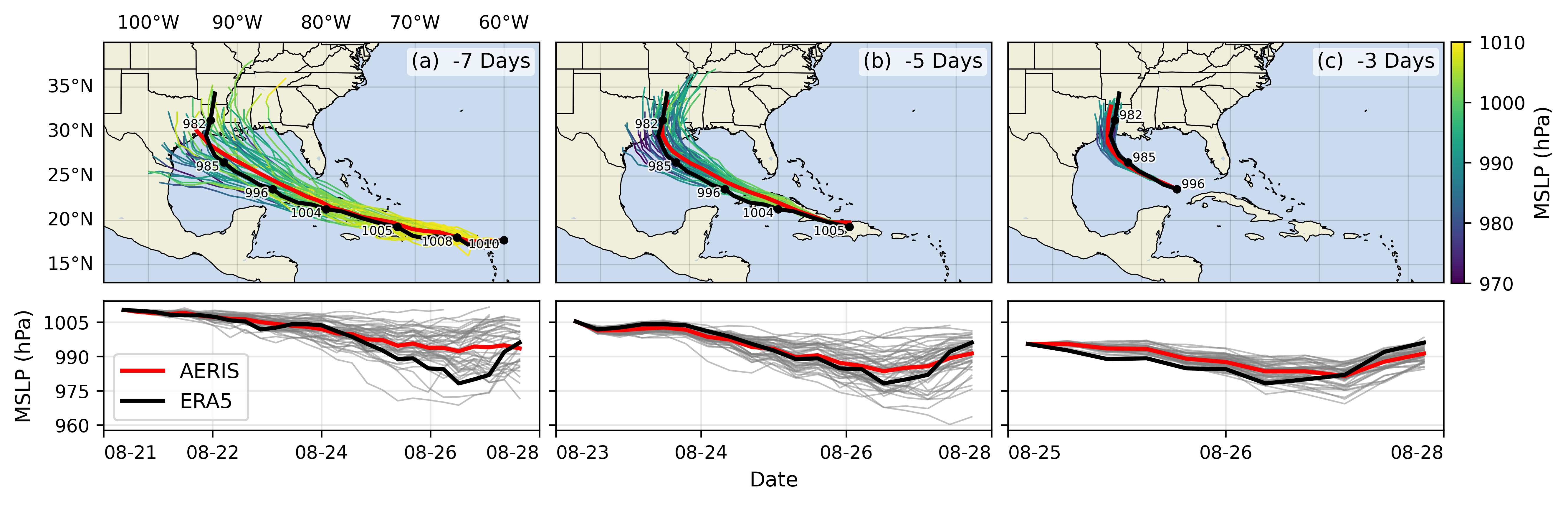
Hurricane Laura

Figure 10: Hurricane Laura tracks (top) and intensity (bottom). Initialized 7(a), 5(b) and 3(c) days prior to 2020-08-28T00z.

S2S: Subsseasonal-to-Seasonal Forecasts

🌡️ S2S Forecasts

We demonstrate for the first time, the ability of a generative, high resolution (native ERA5) diffusion model to produce skillful forecasts on the S2S timescales with realistic evolutions of the Earth system (atmosphere + ocean).

• To assess trends that extend beyond that of our medium-range weather forecasts (beyond 14-days) and evaluate the stability of our model, we made 3,000 forecasts (60 initial conditions each with 50 ensembles) out to 90 days.
• AERIS was found to be stable during these 90-day forecasts
  • Realistic atmospheric states
  • Correct power spectra even at the smallest scales

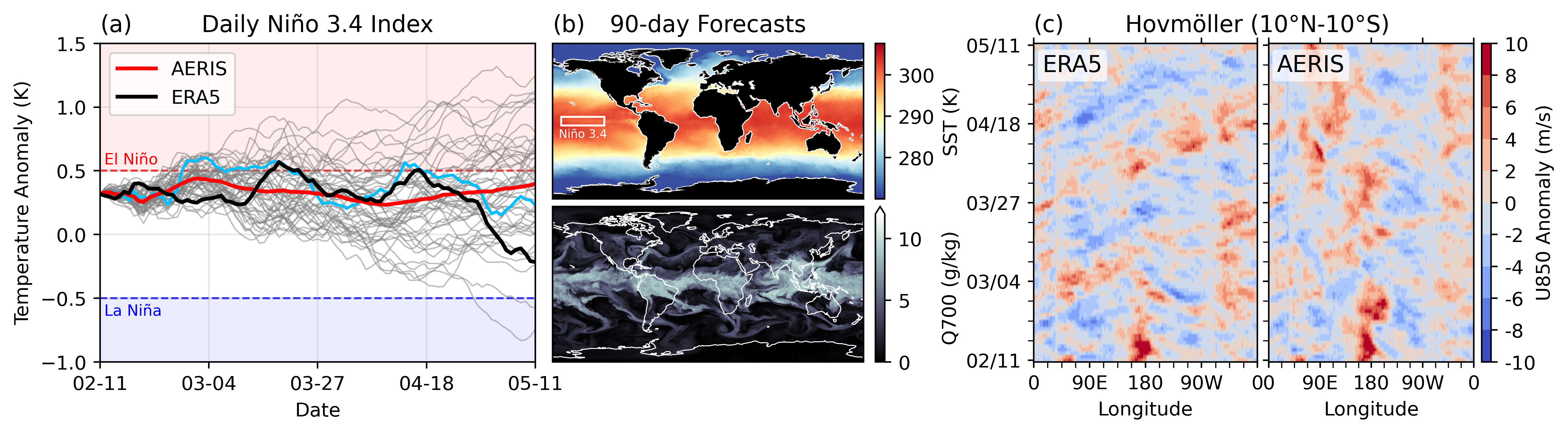
Seasonal Forecast Stability

Figure 11: S2S Stability: (a) Spring barrier El Niño with realistic ensemble spread in the ocean; (b) qualitatively sharp fields of SST and Q700 predicted 90 days in the future from the closest ensemble member to the ERA5 in (a); and (c) stable Hovmöller diagrams of U850 anomalies (climatology removed; m/s), averaged between 10°S and 10°N, for a 90-day rollout.

Next Steps

• Swift: Swift, a single-step consistency model that, for the first time, enables autoregressive finetuning of a probability flow model with a continuous ranked probability score (CRPS) objective

References

1. What are Diffusion Models? | Lil’Log
2. Step by Step visual introduction to Diffusion Models. - Blog by Kemal Erdem
3. Understanding Diffusion Models: A Unified Perspective

Hatanpää, Väinö, Eugene Ku, Jason Stock, Murali Emani, Sam Foreman, Chunyong Jung, Sandeep Madireddy, et al. 2025. “AERIS: Argonne Earth Systems Model for Reliable and Skillful Predictions.” https://arxiv.org/abs/2509.13523.

Price, Ilan, Alvaro Sanchez-Gonzalez, Ferran Alet, Tom R. Andersson, Andrew El-Kadi, Dominic Masters, Timo Ewalds, et al. 2024. “GenCast: Diffusion-Based Ensemble Forecasting for Medium-Range Weather.” https://arxiv.org/abs/2312.15796.

Extras

Overview of Diffusion Models

Goal: We would like to (efficiently) draw samples x_{i} from a (potentially unknown) target distribution q(\cdot).

• Given x_{0} \sim q(x), we can construct a forward diffusion process by gradually adding noise to x_{0} over T steps: x_{0} \rightarrow \left\{x_{1}, \ldots, x_{T}\right\}.

  • Step sizes \beta_{t} \in (0, 1) controlled by a variance schedule \{\beta\}_{t=1}^{T}, with:

    \begin{aligned} q(x_{t}|x_{t-1}) = \mathcal{N}(x_{t}; \sqrt{1-\beta_{t}} x_{t-1}, \beta_{t} I) \\ q(x_{1:T}|x_{0}) = \prod_{t=1}^{T} q(x_{t}|x_{t-1}) \end{aligned}

Diffusion Model: Forward Process

• Introduce:

  • \alpha_{t} \equiv 1 - \beta_{t}
  • \bar{\alpha}_{t} \equiv \prod_{s=1}^{T} \alpha_{s}

  We can write the forward process as:

  q(x_{1}|x_{0}) = \mathcal{N}(x_{1}; \sqrt{\bar{\alpha}_{1}} x_{0}, (1-\bar{\alpha}_{1}) I)

• We see that the mean \mu_{t} = \sqrt{\alpha_{t}} x_{t-1} = \sqrt{\bar{\alpha}_{t}} x_{0}

Acknowledgements

This research used resources of the Argonne Leadership Computing Facility, which is a DOE Office of Science User Facility supported under Contract DE-AC02-06CH11357.