
flowchart LR
    subgraph G0["`GPU0`"]
        subgraph N0["`Network`"]
        end
        L0("`Loss`")
    end
    subgraph D["`Data`"]
        x("`x0`")
        x1("`x1`")
        x2("`x2`")
    end
    x --> N0
    N0 --> L0
    L0 --> N0
classDef block fill:#CCCCCC02,stroke:#838383,stroke-width:1px,color:#838383
classDef eblock fill:#CCCCCC02,stroke:#838383,stroke-width:0px,color:#838383
classDef red fill:#ff8181,stroke:#333,stroke-width:1px,color:#000
classDef green fill:#98E6A5,stroke:#333,stroke-width:1px,color:#000
classDef blue fill:#7DCAFF,stroke:#333,stroke-width:1px,color:#000
classDef grey fill:#cccccc,stroke:#333,stroke-width:1px,color:#000
class x,L0 red
class x1 green
class x2 blue
class x3 grey
class N0,G0,n0 block
class D eblock
Training Foundation Models on Supercomputers
AI
Machine Learning
Supercomputing
A deep dive into the challenges and solutions for training large-scale AI models on supercomputing infrastructure.
🌐 Distributed Training
🚀 Scaling: Overview
- ✅ Goal:
- Minimize: Cost (i.e. amount of time spent training)
- Maximize: Performance
In this talk, we will explore the intricacies of training foundation models on supercomputers. We will discuss the architecture of these models, the computational requirements, and the strategies employed to optimize training processes. Attendees will gain insights into the latest advancements in hardware and software that facilitate efficient model training at scale.
🐢 Training on a Single Device
🕸️ Parallelism Strategies
- Data Parallelism
- Split data across workers
- Easiest to implement
- No changes to model
- Model Parallelism
- Split model across workers
- Hybrid Parallelism
- Combine data + model parallelism
- More complex to implement
- Requires changes to model
👬 Training on Multiple GPUs: Data Parallelism
flowchart LR
    subgraph D["`Data`"]
        direction TB
        x2("`x2`")
        x1("`x1`")
        x("`x0`")
    end
    direction LR
    subgraph G0["`GPU0`"]
        direction LR
        subgraph N0["`NN`"]
        end
        %%y0("`y₀`")
        L0["`Loss`"]
    end
    subgraph G1["`GPU1`"]
        direction LR
        subgraph N1["`NN`"]
        end
        L1["`Loss`"]
    end
    subgraph G2["`GPU2`"]
        direction LR
        subgraph N2["`NN`"]
        end
        L2["`Loss`"]
    end
    x --> N0
    x1 --> N1
    x2 --> N2
    N0 --> L0
    N1 --> L1
    N2 --> L2
classDef block fill:#CCCCCC02,stroke:#838383,stroke-width:1px,color:#838383
classDef eblock fill:#CCCCCC02,stroke:#838383,stroke-width:0px,color:#838383
classDef text fill:#CCCCCC02,stroke:#838383,stroke-width:0px,color:#838383
classDef grey fill:#cccccc,stroke:#333,stroke-width:1px,color:#000
classDef red fill:#ff8181,stroke:#333,stroke-width:1px,color:#000
classDef orange fill:#FFC47F,stroke:#333,stroke-width:1px,color:#000
classDef yellow fill:#FFFF7F,stroke:#333,stroke-width:1px,color:#000
classDef green fill:#98E6A5,stroke:#333,stroke-width:1px,color:#000
classDef blue fill:#7DCAFF,stroke:#333,stroke-width:1px,color:#000
classDef purple fill:#FFCBE6,stroke:#333,stroke-width:1px,color:#000
classDef eblock fill:#CCCCCC02,stroke:#838383,stroke-width:0px,color:#838383
class x,y0,L0 red
class x1,L1 green
class x2,L2 blue
class x3,ar grey
class N0,N1,N2,G0,G1,G2,GU block
class D eblock
class AR block
class bc text
▶️ Data Parallel: Forward Pass
flowchart LR
    subgraph D["`Data`"]
        direction TB
        x("`x0`")
        x1("`x1`")
        x2("`x2`")
    end
    direction LR
    subgraph G0["`GPU0`"]
        direction LR
        subgraph N0["`NN`"]
        end
        L0["`Loss`"]
    end
    subgraph G1["`GPU1`"]
        direction LR
        subgraph N1["`NN`"]
        end
        L1["`Loss`"]
    end
    subgraph G2["`GPU2`"]
        direction LR
        subgraph N2["`NN`"]
        end
        L2["`Loss`"]
    end
    ar("`Avg. Grads<br>(∑ₙgₙ)/N`")
    x --> G0
    x1 --> G1
    x2 --> G2
    N0 --> L0
    N1 --> L1
    N2 --> L2
    L0 -.-> ar
    L1 -.-> ar
    L2 -.-> ar
classDef eblock fill:#CCCCCC02,stroke:#838383,stroke-width:0px,color:#838383
classDef block fill:#CCCCCC02,stroke:#838383,stroke-width:1px,color:#838383
classDef grey fill:#cccccc,stroke:#333,stroke-width:1px,color:#000
classDef red fill:#ff8181,stroke:#333,stroke-width:1px,color:#000
classDef orange fill:#FFC47F,stroke:#333,stroke-width:1px,color:#000
classDef yellow fill:#FFFF7F,stroke:#333,stroke-width:1px,color:#000
classDef green fill:#98E6A5,stroke:#333,stroke-width:1px,color:#000
classDef blue fill:#7DCAFF,stroke:#333,stroke-width:1px,color:#000
classDef purple fill:#FFCBE6,stroke:#333,stroke-width:1px,color:#000
classDef text fill:#CCCCCC02,stroke:#838383,stroke-width:0px,color:#838383
class x,y0,L0 red
class x1,L1 green
class x2,L2 blue
class x3,ar grey
class N0,N1,N2,G0,G1,G2,GU block
class D eblock
class AR block
class bc text
◀️ Data Parallel: Backward Pass
flowchart RL
    subgraph D["`Data`"]
        direction TB
        x("`x0`")
        x1("`x1`")
        x2("`x1`")
    end
    subgraph G0["`GPU0`"]
        direction RL
        subgraph N0["`NN`"]
        end
        L0["`Loss`"]
    end
    subgraph G1["`GPU1`"]
        direction RL
        subgraph N1["`NN`"]
        end
        L1["`Loss`"]
    end
    subgraph G2["`GPU2`"]
        direction RL
        subgraph N2["`NN`"]
        end
        L2["`Loss`"]
    end
    subgraph BC["`Send Updates`"]
        direction TB
    end
    BC -.-> G0
    BC -.-> G1
    BC -.-> G2
    L0 ~~~ N0
    L1 ~~~ N1
    L2 ~~~ N2
    G0 ~~~ x
    G1 ~~~ x1
    G2 ~~~ x2
classDef grey fill:#cccccc,stroke:#333,stroke-width:1px,color:#000
classDef eblock fill:#CCCCCC02,stroke:#838383,stroke-width:0px,color:#838383
classDef block fill:#CCCCCC02,stroke:#838383,stroke-width:1px,color:#838383
classDef red fill:#ff8181,stroke:#333,stroke-width:1px,color:#000
classDef orange fill:#FFC47F,stroke:#333,stroke-width:1px,color:#000
classDef yellow fill:#FFFF7F,stroke:#333,stroke-width:1px,color:#000
classDef green fill:#98E6A5,stroke:#333,stroke-width:1px,color:#000
classDef blue fill:#7DCAFF,stroke:#333,stroke-width:1px,color:#000
classDef purple fill:#FFCBE6,stroke:#333,stroke-width:1px,color:#000
classDef text fill:#CCCCCC02,stroke:#838383,stroke-width:0px,color:#838383
class x,y0,L0 red
class x1,L1 green
class x2,L2 blue
class x3,ar grey
class N0,N1,N2,G0,G1,G2,GU block
class BC block
class bc text
class D eblock
🔄 Collective Communication
- Broadcast: Send data from one node to all other nodes
- Reduce: Aggregate data from all nodes to one node
- AllReduce: Aggregate data from all nodes to all nodes
- Gather: Collect data from all nodes to one node
- AllGather: Collect data from all nodes to all nodes
- Scatter: Distribute data from one node to all other nodes
Reduce
- Perform a reduction on data across ranks, send to individual
flowchart TD
  subgraph R0["`0`"]
    x0("`x0`")
  end
  subgraph R1["`1`"]
    x1("`x1`")
  end
  subgraph R2["`2`"]
    x2("`x2`")
  end
  subgraph R3["`3`"]
    x3("`x3`")
  end
  subgraph AR["`Reduce`"]
    xp["`z=reduce(x, 2, SUM)`"]
  end
  subgraph AR3["`3`"]
  end
  subgraph AR2["`2`"]
    xp2("`z`")
  end
  subgraph AR1["`1`"]
  end
  subgraph AR0["`0`"]
  end
  x0 --> AR
  x1 --> AR
  x2 --> AR
  x3 --> AR
  AR --> AR3
  AR --> xp2
  AR --> AR1
  AR --> AR0
classDef block fill:#CCCCCC02,stroke:#838383,stroke-width:1px,color:#838383
classDef red fill:#ff8181,stroke:#333,stroke-width:1px,color:#000
classDef orange fill:#FFC47F,stroke:#333,stroke-width:1px,color:#000
classDef green fill:#98E6A5,stroke:#333,stroke-width:1px,color:#000
classDef yellow fill:#FFFF7F,stroke:#333,stroke-width:1px,color:#000
classDef blue fill:#7DCAFF,stroke:#333,stroke-width:1px,color:#000
classDef purple fill:#FFCBE6,stroke:#333,stroke-width:1px,color:#000
classDef pink fill:#E599F7,stroke:#333,stroke-width:1px,color:#000
class R0,R1,R2,R3,AR,AR0,AR1,AR2,AR3 block
class xp,xp2 purple
class x0 red
class x1 green
class x2 blue
class x3 yellow
🐣 Getting Started: In Practice
- 📦 Distributed Training Frameworks:
- 🍋 saforem2 /
ezpz - 🤖 Megatron-LM
- 🤗 Accelerate
- 🔥 PyTorch
- 🍋 saforem2 /
- 🚀 DeepSpeed
- 🧠 Memory Management:
- FSDP vs. ZeRO
- Activation Checkpointing
- Mixed Precision Training
- Gradient Accumulation
- Offloading to CPU/NVMe
📝 Plan of Attack
flowchart TB
    A{"Model Perfect?"}
    A -- no --> M{"Available Memory?"}
    A -- yes --> AD["Done"]
    M -- yes --> MY["Make Model Larger"]
    M -- no --> ZMP["<b>Free Up Memory</b>"]
    MY --> A
    ZMP --> MY
    A:::block
    M:::block
    AD:::block
    MY:::block
    ZMP:::sblock
    classDef text fill:#CCCCCC02,stroke:#838383,stroke-width:0px,color:#838383
    classDef sblock fill:#CCCCCC02,stroke:#838383,stroke-width:1px,color:#838383,white-space:collapse
    classDef block fill:#CCCCCC02,stroke:#838383,stroke-width:1px,color:#838383
🚀 Going Beyond Data Parallelism
- ✅ Useful when model fits on single GPU:
- ultimately limited by GPU memory
- model performance limited by size
- ⚠️ When model does not fit on a single GPU:
- Offloading (can only get you so far…):
- Otherwise, resort to model parallelism strategies
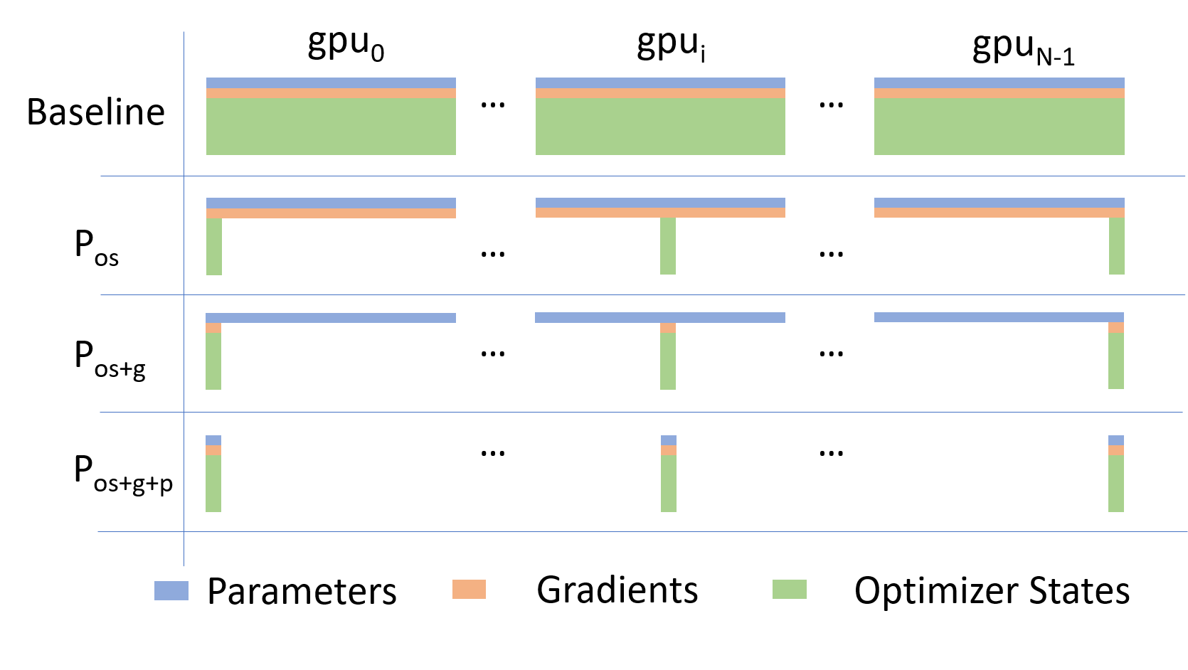
Going beyond Data Parallelism: ZeRO
- Depending on the
ZeROstage (1, 2, 3), we can offload:- Stage 1: optimizer states \left(P_{\mathrm{os}}\right)
- Stage 2: gradients + opt. states \left(P_{\mathrm{os}+\mathrm{g}}\right)
- Stage 3: model params + grads + opt. states \left(P_{\mathrm{os}+\mathrm{g}+\mathrm{p}}\right)
🕸️ Additional Parallelism Strategies
- Tensor (/ Model) Parallelism (
TP): - Pipeline Parallelism (
PP): - Sequence Parallelism (
SP): -
- Supports 4D Parallelism (
DP+TP+PP+SP)
- Supports 4D Parallelism (
Pipeline Parallelism (PP)
- Model is split up vertically (layer-level) across multiple GPUs
- Each GPU:
- has a portion of the full model
- processes in parallel different stages of the pipeline (on a small chunk of the batch)
- See:
flowchart TB
    subgraph G0["`GPU 0`"]
        direction LR
        a0("`Layer 0`")
        b0("`Layer 1`")
    end
    subgraph G1["`GPU 1`"]
        direction LR
        a1("`Layer 2`")
        b1("`Layer 3`")
    end
    a0 -.-> b0
    b0 --> a1
    a1 -.-> b1
classDef block fill:#CCCCCC02,stroke:#838383,stroke-width:1px,color:#838383
classDef red fill:#ff8181,stroke:#333,stroke-width:1px,color:#000
classDef orange fill:#FFC47F,stroke:#333,stroke-width:1px,color:#000
classDef yellow fill:#FFFF7F,stroke:#333,stroke-width:1px,color:#000
classDef green fill:#98E6A5,stroke:#333,stroke-width:1px,color:#000
classDef blue fill:#7DCAFF,stroke:#333,stroke-width:1px,color:#000
classDef purple fill:#FFCBE6,stroke:#333,stroke-width:1px,color:#000
class G0,G1 block
class a0 red
class b0 green
class a1 blue
class b1 yellow
Tensor Parallel (TP)
- Each tensor is split up into multiple chunks
- Each shard of the tensor resides on its designated GPU
- During processing each shard gets processed separately (and in parallel) on different GPUs
- synced at the end of the step
- See: 🤗 Model Parallelism for additional details
flowchart LR
   subgraph G0["`GPU0`"]
    direction TB
    a0("`Layer 0`")
    b0("`Layer 1`")
    c0("`Layer 2`")
    d0("`Layer 3`")
   end
   subgraph G1["`GPU1`"]
    direction TB
    a1("`Layer 0`")
    b1("`Layer 1`")
    c1("`Layer 2`")
    d1("`Layer 3`")
   end
   a0 <-.-> a1
   b0 <-.-> b1
   c0 <-.-> c1
   d0 <-.-> d1
classDef red fill:#ff8181,stroke:#333,stroke-width:1px,color:#000
classDef orange fill:#FFC47F,stroke:#333,stroke-width:1px,color:#000
classDef yellow fill:#FFFF7F,stroke:#333,stroke-width:1px,color:#000
classDef green fill:#98E6A5,stroke:#333,stroke-width:1px,color:#000
classDef blue fill:#7DCAFF,stroke:#333,stroke-width:1px,color:#000
classDef purple fill:#FFCBE6,stroke:#333,stroke-width:1px,color:#000
classDef block fill:#CCCCCC02,stroke:#838383,stroke-width:1px,color:#838383
class G0,G1 block
class a0,a1 red
class b0,b1 green
class c0,c1 blue
class d0,d1 yellow
Tensor Parallel (TP)
- Suitable when the model is too large to fit onto a single device (CPU / GPU)
- Typically more complicated to implement than data parallel training
- This is what one may call horizontal parallelism
- Communication whenever dataflow between two subsets
-
argonne-lcf/Megatron-DeepSpeed - 🤗
huggingface/nanotron
flowchart LR
   subgraph G0["`GPU0`"]
    direction TB
    a0("`Layer 0`")
    b0("`Layer 1`")
    c0("`Layer 2`")
    d0("`Layer 3`")
   end
   subgraph G1["`GPU1`"]
    direction TB
    a1("`Layer 0`")
    b1("`Layer 1`")
    c1("`Layer 2`")
    d1("`Layer 3`")
   end
   a0 <-.-> a1
   b0 <-.-> b1
   c0 <-.-> c1
   d0 <-.-> d1
classDef red fill:#ff8181,stroke:#333,stroke-width:1px,color:#000
classDef orange fill:#FFC47F,stroke:#333,stroke-width:1px,color:#000
classDef yellow fill:#FFFF7F,stroke:#333,stroke-width:1px,color:#000
classDef green fill:#98E6A5,stroke:#333,stroke-width:1px,color:#000
classDef blue fill:#7DCAFF,stroke:#333,stroke-width:1px,color:#000
classDef purple fill:#FFCBE6,stroke:#333,stroke-width:1px,color:#000
classDef block fill:#CCCCCC02,stroke:#838383,stroke-width:1px,color:#838383
class G0,G1 block
class a0,a1 red
class b0,b1 green
class c0,c1 blue
class d0,d1 yellow
- Split up network over multiple workers
- Each receives disjoint subset
- All communication associated with subsets are distributed
- Communication whenever dataflow between two subsets
- Typically more complicated to implement than data parallel training
- Suitable when the model is too large to fit onto a single device (CPU / GPU)
Tensor (/ Model) Parallel Training: Example
Want to compute: y = \sum_{i} x_{i} W_{i} = x_0 * W_0 + x_1 * W_1 + x_2 * W_2
where each GPU has only its portion of the full weights as shown below
- Compute: y_{0} = x_{0} * W_{0}\rightarrow
GPU1 - Compute: y_{1} = y_{0} + x_{1} * W_{1}\rightarrow
GPU2 - Compute: y = y_{1} + x_{2} * W_{2} = \sum_{i} x_{i} W_{i} ✅
flowchart LR
    subgraph X0["`GPU0`"]
        direction LR
        a("`W0`")
    end
    subgraph X1["`GPU1`"]
        direction LR
        b("`W1`")
    end
    subgraph X2["`GPU2`"]
        direction LR
        c("`W2`")
    end
  t0("`x0`")-->X0
  X0 -->|"`x0 W0`"|X1
  X1 -->|"`x0 W0 <br>+ x1 W1`"|X2
  t1("`x1`") --> X1
  t2("`x1`") --> X2
🔭 AI-for-Science
ChatGPT: explain this image
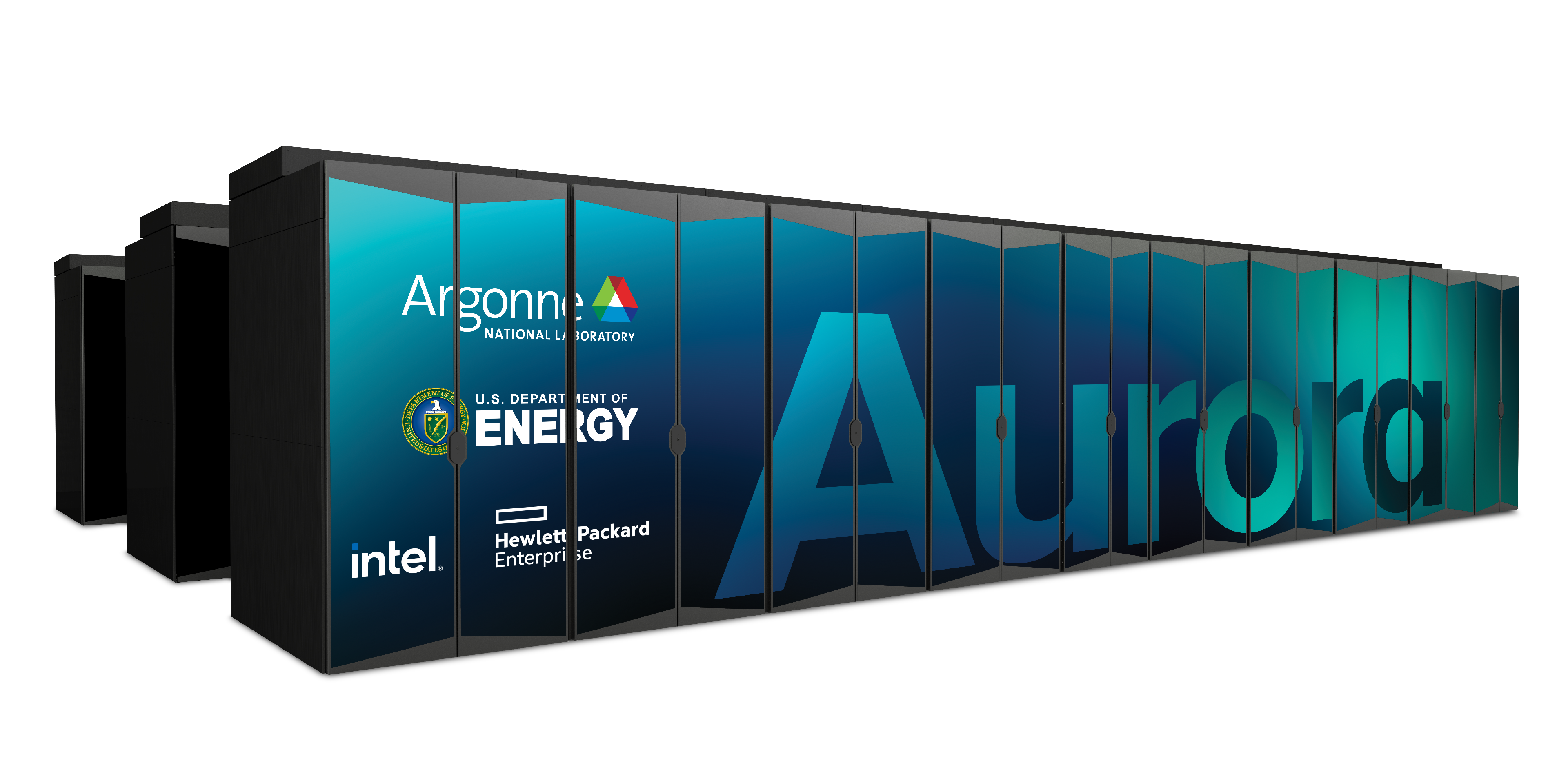
🏗️ Aurora
🌌 AuroraGPT (2024–)
AuroraGPT: General purpose scientific LLM Broadly trained on a general corpora plus scientific {papers, texts, data}
- Explore pathways towards a “Scientific Assistant” model
- Build with international partners (RIKEN, BSC, others)
- Multilingual English, 日本語, French, German, Spanish
- Multimodal: images, tables, equations, proofs, time series, graphs, fields, sequences, etc

Awesome-LLM
🧪 AuroraGPT: Open Science Foundation Model

🧰 AuroraGPT: Toolbox
- Datasets and data pipelines (how do we deal with scientific data?)
- Software infrastructure and workflows (scalable, robust, extensible)
- Evaluation of state-of-the-art LLM Models (how do they perform on scientific tasks?)
🏋️ Challenges: In Practice
This is incredibly difficult in practice, due in part to:
- Brand new {hardware, architecture, software}
- Lack of native support in existing frameworks (though getting better!)
- General system stability
+10k Nodes \left(\times \frac{12\,\,\mathrm{XPU}}{1\,\,\mathrm{Node}}\right)\Rightarrow +100k XPUs- network performance
- file system stability (impacted by other users !)
- many unexpected difficulties occur at increasingly large scales
- Combinatorial explosion of possible configurations and experiments
- {hyperparameters, architectures, tokenizers, learning rates, …}
💾 AuroraGPT: Training
- To train a fixed model on trillions of tokens requires:
- Aggregating data from multiple different corpora
(e.g. ArXiv, Reddit, StackExchange, GitHub, Wikipedia, etc.) - Sampling each training batch according to a fixed distribution across corpora
- Building indices that map batches of tokens into these files (indexing)
The original implementation was slow:
- Designed to run serially on a single device
- Major bottleneck when debugging data pipeline at scale
- Aggregating data from multiple different corpora
🍹 AuroraGPT: Blending Data, Efficiently
- 🐢 Original implementation:
- Slow (serial, single device)
- ~ 1 hr/2T tokens
- 🐇 New implementation:
- Fast! (distributed, asynchronous)
- ~ 2 min/2T tokens
(30x faster !!)

📉 Loss Curve: Training AuroraGPT-7B on 2T Tokens

✨ Features
- 🕸️ Parallelism:
- {data, tensor, pipeline, sequence, …}
- ♻️ Checkpoint Converters:
- Megatron ⇄ 🤗 HF ⇄ ZeRO ⇄ Universal
- 🔀 DeepSpeed Integration:
- ZeRO Offloading
- Activation checkpointing
- AutoTP (WIP)
- ability to leverage features from DeepSpeed community
✨ Features (even more!)
🧬 MProt-DPO
- Finalist: SC’24 ACM Gordon Bell Prize
- One of the first protein design toolkits that integrates:
- Text, (protein/gene) sequence, structure/conformational sampling modalities to build aligned representations for protein sequence-function mapping
🧬 Scaling Results (2024)

3.5B model across ~38,400 GPUs
~ 4 EFLOPS @ Aurora
38,400 XPUs
= 3200 [node] x 12 [XPU / node]
This novel work presents a scalable, multimodal workflow for protein design that trains an LLM to generate protein sequences, computationally evaluates the generated sequences, and then exploits them to fine-tune the model.
Direct Preference Optimization steers the LLM toward the generation of preferred sequences, and enhanced workflow technology enables its efficient execution. A 3.5B and a 7B model demonstrate scalability and exceptional mixed precision performance of the full workflow on ALPS, Aurora, Frontier, Leonardo and PDX.
🧬 MProt-DPO: Scaling Results
3.5B model

7B model
🚂 Loooooooooong Sequence Lengths

![]()
- Working with Microsoft/DeepSpeed team to enable longer sequence lengths (context windows) for LLMs
- See my blog post for additional details


SEQ_LEN for both 25B and 33B models (See: Song et al. (2023))
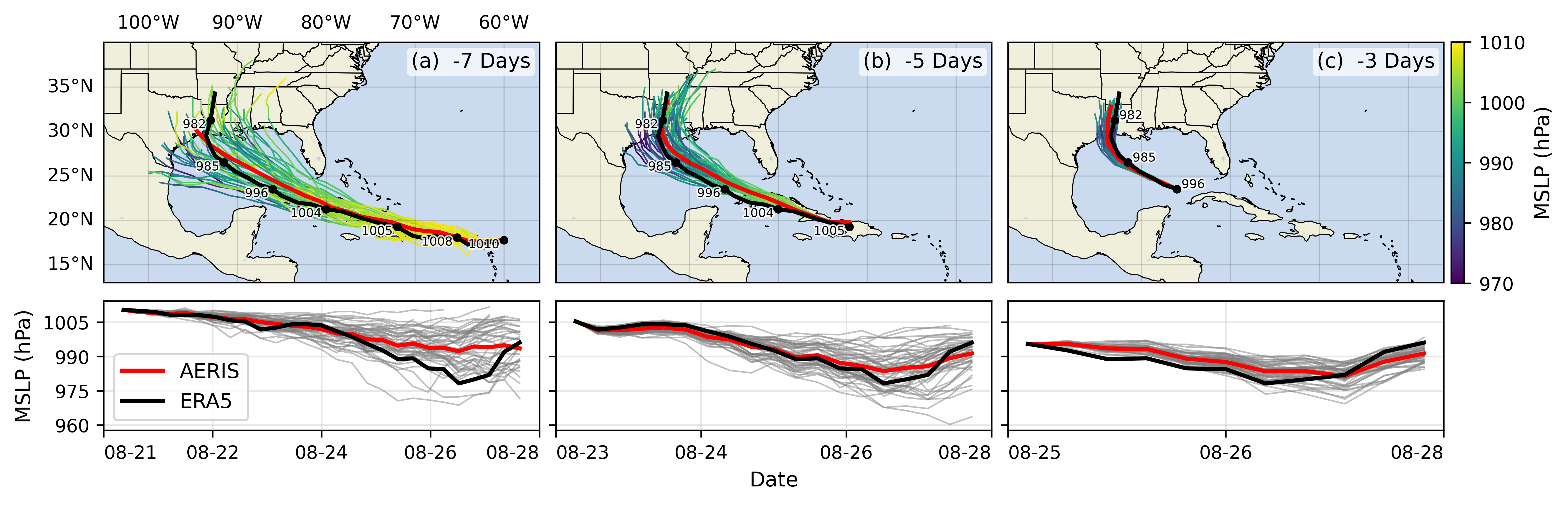
🌎 AERIS (2025)
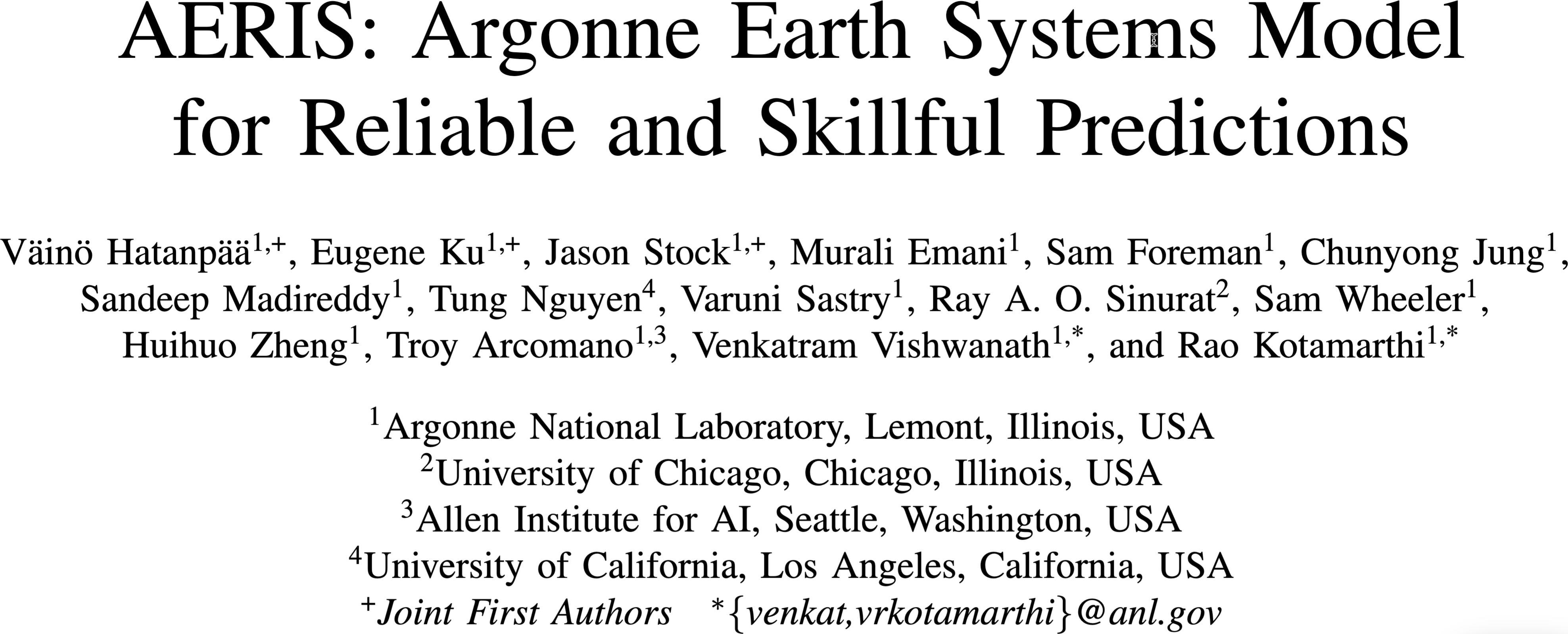

We demonstrate a significant advancement in AI weather and climate modeling with AERIS by efficient scaling of window-based transformer models. We have performed global medium-range forecasts with performance competitive with GenCast and surpassing the IFS ENS model, with longer, 90- day rollouts showing our ability to learn atmospheric dynamics on seasonal scales without collapsing, becoming the first diffusion-based model that can work across forecast scales from 6 hours all the way to 3 months with remarkably accurate out of distribution predictions of extreme events.
👀 High-Level Overview of AERIS
| Property | Description |
|---|---|
| Domain | Global |
| Resolution | 0.25° & 1.4° |
| Training Data | ERA5 (1979–2018) |
| Model Architecture | Swin Transformer |
| Speedup4 | O(10k–100k) |
➕ Contributions
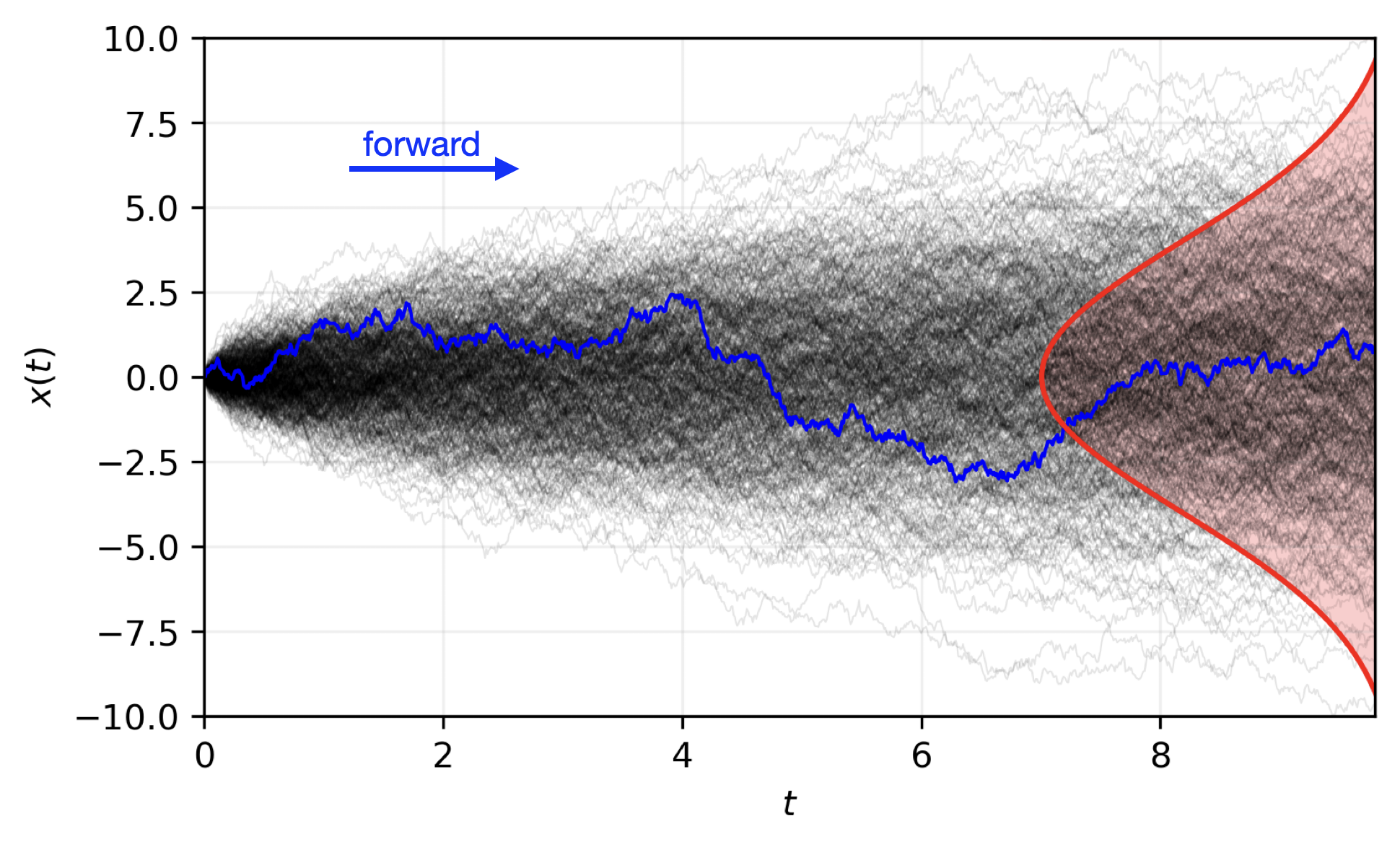
⚠️ Issues with the Deterministic Approach
Transformers: - Deterministic
- Single input → single forecast
Diffusion: - Probabilistic
- Single input → ensemble of forecasts
- Captures uncertainty and variability in weather predictions
- Enables ensemble forecasting for better risk assessment
🎲 Transitioning to a Probabilistic Model

🌀 Sequence-Window-Pipeline Parallelism SWiPe
SWiPeis a novel parallelism strategy for Swin-based Transformers- Hybrid 3D Parallelism strategy, combining:
- Sequence parallelism (
SP) - Window parallelism (
WP) - Pipeline parallelism (
PP)
- Sequence parallelism (


SWiPe Communication Patterns
🚀 AERIS: Scaling Results

- 10 EFLOPs (sustained) @ 120,960 GPUs
- See (Hatanpää et al. (2025)) for additional details
- arXiv:2509.13523
🌪️ Hurricane Laura
📓 References
Hatanpää, Väinö, Eugene Ku, Jason Stock, et al. 2025. AERIS: Argonne Earth Systems Model for Reliable and Skillful Predictions. https://arxiv.org/abs/2509.13523.
Price, Ilan, Alvaro Sanchez-Gonzalez, Ferran Alet, et al. 2024. GenCast: Diffusion-Based Ensemble Forecasting for Medium-Range Weather. https://arxiv.org/abs/2312.15796.
Song, Shuaiwen Leon, Bonnie Kruft, Minjia Zhang, et al. 2023. DeepSpeed4Science Initiative: Enabling Large-Scale Scientific Discovery Through Sophisticated AI System Technologies. https://arxiv.org/abs/2310.04610.
❤️ Acknowledgements
This research used resources of the Argonne Leadership Computing Facility, which is a DOE Office of Science User Facility supported under Contract DE-AC02-06CH11357.
Footnotes
Each node has 6 Intel Data Center GPU Max 1550 (code-named “Ponte Vecchio”) tiles, with 2 XPUs per tile.↩︎
Implemented by Marieme Ngom↩︎
GenCast: A Generative Model for Medium-Range Global Weather Forecasting (Price et al. (2024))↩︎
Demonstrated on up to 120,960 GPUs on Aurora and 8,064 GPUs on LUMI.↩︎
Citation
BibTeX citation:
@unpublished{foreman2025,
  author = {Foreman, Sam},
  title = {Training {Foundation} {Models} on {Supercomputers}},
  date = {2025-10-15},
  url = {https://samforeman.me/talks/2025/10/15/slides.html},
  langid = {en}
}
For attribution, please cite this work as:
Foreman, Sam. 2025. “Training Foundation Models on
Supercomputers.” October 15. https://samforeman.me/talks/2025/10/15/slides.html.